지난주 감성 분류기는 토큰 임베딩을 그냥 평균 냈다. 평균은 순서도, 중요도도 모른다. 오늘은 어떤 토큰을 얼마나 볼지 모형이 스스로 정하게 만든다.
\[S = \frac{QK^\top}{\sqrt{d}} \;\to\; \text{mask} \;\to\; W = \text{softmax}(S) \;\to\; WV\]
이론에서 손으로 계산한 그 값들을 코드로 한 줄씩 재현하고 F.scaled_dot_product_attention 과 대조한 뒤, 어텐션을 쓴 감성 분류기를 학습 시켜 모형이 문장의 어느 단어를 봤는지 꺼내 본다.
\(Q, K, V\) 만들기세 가지 역할 (Ch11)
스코어 \(QK^\top\) · \(\sqrt{d}\) 스케일링
어텐션 손계산 (a)(b) (Ch11)
행별 Softmax · 가중합
어텐션 손계산 (c)(d) (Ch11)
인과 마스크 (\(-\infty\) )
인과 마스크 손계산 (Ch11)
head 분할 · 결합
Multi-Head 모양 추적 (Ch11)
파라미터 \(4d^2\)
head 수와 무관 (Ch11)
F.scaled_dot_product_attention직접 만든 것과 대조
1. 손계산 그대로 재현하기
Ch11에서 토큰 3개짜리 문장 “고양이가 / 생선을 / 먹었다”로 계산했던 그 값이다.
import numpy as npimport pandas as pdimport torchimport torch.nn as nnimport torch.nn.functional as Fimport matplotlib.pyplot as plt= 4 , sci_mode= False )42 )= ['고양이가' , '생선을' , '먹었다' ]= torch.tensor([[2. , 1. ], [1. , 2. ], [1. , 3. ]])= torch.tensor([[1. , 0. ], [0. , 2. ], [1. , 1. ]])= torch.tensor([[1. , 0. ], [0. , 1. ], [1. , 1. ]])print ('Q shape:' , tuple (Q.shape), ' (토큰 수, d)' )print (pd.DataFrame({'토큰' : tokens,'q' : [tuple (v.tolist()) for v in Q],'k' : [tuple (v.tolist()) for v in K],'v' : [tuple (v.tolist()) for v in V]}).to_string(index= False ))
Q shape: (3, 2)  (토큰 수, d)
  토큰          q          k          v
고양이가 (2.0, 1.0) (1.0, 0.0) (1.0, 0.0)
 생선을 (1.0, 2.0) (0.0, 2.0) (0.0, 1.0)
 먹었다 (1.0, 3.0) (1.0, 1.0) (1.0, 1.0)
1-1. (a) 스코어 — 모든 쌍의 내적
= Q @ K.Tprint ('shape :' , tuple (S.shape), ' (Query 수, Key 수)' )print (pd.DataFrame(S.numpy(), index= [f' { t} 의 q' for t in tokens],= [f' { t} 의 k' for t in tokens]))
shape : (3, 3)  (Query 수, Key 수)
         고양이가의 k  생선을의 k  먹었다의 k
고양이가의 q      2.0     2.0     3.0
생선을의 q       1.0     4.0     3.0
먹었다의 q       1.0     6.0     4.0
“먹었다” 행이 (1, 6 , 4)다 — “먹었다”의 Query가 “생선을”의 Key와 가장 잘 맞는다. 한 칸만 손으로 확인해 본다.
print ('q(먹었다) · k(생선을) =' , float (Q[2 ] @ K[1 ]), ' = 1x0 + 3x2' )
q(먹었다) · k(생선을) = 6.0 = 1x0 + 3x2
1-2. (b) \(\sqrt{d}\) 로 나누기
= Q.shape[1 ]= S / (d ** 0.5 )print ('d =' , d, ' sqrt(d) =' , round (d** 0.5 , 4 ))print (pd.DataFrame(S_scaled.numpy().round (2 ), index= tokens, columns= tokens))
d = 2   sqrt(d) = 1.4142
      고양이가   생선을   먹었다
고양이가  1.41  1.41  2.12
생선을   0.71  2.83  2.12
먹었다   0.71  4.24  2.83
차원이 커지면 내적 값 자체가 커지고, Softmax가 한 곳에 확률을 몰아준다. \(\sqrt{d}\) 로 나누는 것은 그 안전장치다.
1-3. (c) 행별 Softmax
= S_scaled.softmax(dim=- 1 ) # 마지막 축(Key 방향)으로 softmax print (pd.DataFrame(W.numpy().round (3 ), index= tokens, columns= tokens))print (' \n 각 행의 합 :' , W.sum (dim=- 1 ).numpy())
       고양이가    생선을    먹었다
고양이가  0.248  0.248  0.503
생선을   0.074  0.620  0.306
먹었다   0.023  0.786  0.191

각 행의 합 : [1. 1. 1.]
Softmax는 행마다 독립적으로 걸려야 한다. 한 Query가 여러 Key에 나눠 주는 가중치의 합이 1이 되는 것이지, 열 방향 합이 1이 되는 것이 아니다.
3주차의 keepdims 문제와 같은 자리다 — 어느 축으로 정규화하는가 를 항상 확인한다.
# 직접 계산해서 확인 — "먹었다" 행 = S_scaled[2 ]= torch.exp(row - row.max ())print ('exp :' , e.numpy().round (4 ))print ('합 :' , float (e.sum ()).__round__ (4 ))print ('직접 :' , (e / e.sum ()).numpy().round (4 ))print ('softmax:' , W[2 ].numpy().round (4 ))
exp    : [0.0291 1.     0.2431]
합     : 1.2723
직접   : [0.0229 0.786  0.1911]
softmax: [0.0229 0.786  0.1911]
1-4. (d) 가중합 — 새 표현 벡터
= W @ Vprint ('shape :' , tuple (out.shape))print (pd.DataFrame(out.numpy().round (4 ), index= tokens, columns= ['성분1' , '성분2' ]))
shape : (3, 2)
         성분1     성분2
고양이가  0.7517  0.7517
생선을   0.3800  0.9257
먹었다   0.2140  0.9771
“먹었다”의 새 표현은 (0.214, 0.977)이다. Value의 두 성분을 “동물 성분 / 음식 성분”으로 읽으면, “먹었다”가 음식 쪽으로 강하게 끌려간 것 이 보인다. 가중치의 0.786이 “생선을”에 갔기 때문이다.
가중치 행렬 W 의 1행이 (0.248, 0.248, 0.503) 이다. 이 가중치로 V 를 가중합해 “고양이가”의 새 표현을 직접 계산 하시오.
= W[0 ] # (0.248, 0.248, 0.503) = None # ← w_row 와 V 로 가중합을 만드세요 assert new_repr is not None and tuple (new_repr.shape) == (2 ,), '모양을 확인하세요' assert torch.allclose(new_repr, out[0 ], atol= 1e-4 ), '값이 다릅니다' print ('통과' , new_repr.numpy().round (4 ))
정답 코드 보기
= W[0 ]= (w_row.unsqueeze(1 ) * V).sum (0 ) # 또는 w_row @ V print ('가중합 :' , new_repr.numpy().round (4 ))print ('W @ V :' , out[0 ].numpy().round (4 ))print ('성분 1 =' , ' + ' .join(f' { float (w_row[i]):.3f} x { float (V[i,0 ]):.0f} ' for i in range (3 )))
가중합 : [0.7517 0.7517]
W @ V  : [0.7517 0.7517]
성분 1 = 0.248x1 + 0.248x0 + 0.503x1
1-5. 함수 하나로 묶고, PyTorch와 대조
def attention(Q, K, V, mask= None ):= Q.shape[- 1 ]= Q @ K.transpose(- 2 , - 1 ) / (d ** 0.5 )if mask is not None := S.masked_fill(mask, float ('-inf' ))= S.softmax(dim=- 1 )return W @ V, W= attention(Q, K, V)= F.scaled_dot_product_attention(Q, K, V)print ('직접 구현: \n ' , mine.numpy().round (4 ))print (' \n PyTorch : \n ' , ref.numpy().round (4 ))print (' \n 일치:' , torch.allclose(mine, ref, atol= 1e-6 ))
직접 구현:
 [[0.7517 0.7517]
 [0.38   0.9257]
 [0.214  0.9771]]

PyTorch  :
 [[0.7517 0.7517]
 [0.38   0.9257]
 [0.214  0.9771]]

일치: True
2. 인과 마스크 — 미래를 보면 안 된다
2-1. 마스크 만들기
= 3 = torch.triu(torch.ones(T, T, dtype= torch.bool ), diagonal= 1 )print ('mask (True = 가릴 자리): \n ' , mask.numpy())
mask (True = 가릴 자리):
 [[False  True  True]
 [False False  True]
 [False False False]]
diagonal=1 은 대각선 위쪽 만 True로 만든다. 자기 자신(대각선)은 볼 수 있어야 한다.
2-2. \(-\infty\) 를 넣고 Softmax
= S_scaled.masked_fill(mask, float ('-inf' ))print ('마스크 적용 후 스코어: \n ' , S_masked.numpy())= S_masked.softmax(dim=- 1 )print (' \n 가중치:' )print (pd.DataFrame(W_causal.numpy().round (3 ), index= tokens, columns= tokens))print (' \n 각 행의 합:' , W_causal.sum (- 1 ).numpy())
마스크 적용 후 스코어:
 [[1.4142135        -inf       -inf]
 [0.70710677 2.828427         -inf]
 [0.70710677 4.242641   2.828427  ]]

가중치:
       고양이가    생선을    먹었다
고양이가  1.000  0.000  0.000
생선을   0.107  0.893  0.000
먹었다   0.023  0.786  0.191

각 행의 합: [1. 1. 1.]
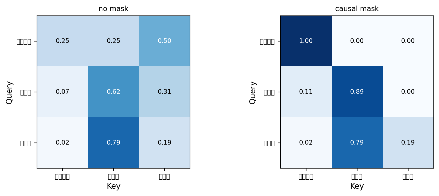
Ch11에서 손으로 구한 표와 같다 — 1행 1.000, 2행 (0.107, 0.893), 3행 (0.023, 0.786, 0.191). 아래쪽 삼각형만 남았고, 각 행의 합은 여전히 1 이다.
# 2행을 손으로 확인 print ('e^0.71 =' , round (float (torch.exp(S_scaled[1 ,0 ])), 3 ))print ('e^2.83 =' , round (float (torch.exp(S_scaled[1 ,1 ])), 3 ))= float (torch.exp(S_scaled[1 ,0 ]) + torch.exp(S_scaled[1 ,1 ]))print ('합 =' , round (tot, 3 ))print ('가중치 =' , round (float (torch.exp(S_scaled[1 ,0 ]))/ tot, 3 ),round (float (torch.exp(S_scaled[1 ,1 ]))/ tot, 3 ))
e^0.71 = 2.028
e^2.83 = 16.919
합     = 18.947
가중치 = 0.107 0.893
2-3. 왜 0을 곱하지 않고 \(-\infty\) 를 넣는가
# 잘못된 방법: softmax 뒤에 0을 곱한다 = W.clone()= 0.0 print ('softmax 뒤에 0을 곱한 경우:' )print (pd.DataFrame(W_wrong.numpy().round (3 ), index= tokens, columns= tokens))print ('행의 합:' , W_wrong.sum (- 1 ).numpy(), ' ← 1이 아니다' )print ()print ('softmax 전에 -inf를 넣은 경우 행의 합:' , W_causal.sum (- 1 ).numpy())
softmax 뒤에 0을 곱한 경우:
       고양이가    생선을    먹었다
고양이가  0.248  0.000  0.000
생선을   0.074  0.620  0.000
먹었다   0.023  0.786  0.191
행의 합: [0.24825507 0.6943047  1.        ]  ← 1이 아니다

softmax 전에 -inf를 넣은 경우 행의 합: [1. 1. 1.]
가려야 할 자리는 Softmax를 계산하기 전에 없애야 한다. 나중에 0을 곱하면 남은 가중치의 합이 1이 되지 않는다.
토큰이 5개일 때, 자기 자신과 그 이전만 보는 인과 마스크를 만드시오. torch.triu 를 쓰되 diagonal 값을 스스로 정해 보라.
= None # ← (5, 5) bool 텐서, True = 가릴 자리 assert mask5 is not None and mask5.shape == (5 , 5 )assert mask5.diagonal().sum () == 0 , '자기 자신은 봐야 합니다' assert mask5.sum () == 10 , f'가리는 칸 수가 다릅니다: { int (mask5.sum ())} ' print ('통과 \n ' , mask5.numpy().astype(int ))
정답 코드 보기
= torch.triu(torch.ones(5 , 5 , dtype= torch.bool ), diagonal= 1 )print (mask5.numpy().astype(int ))print ('가리는 칸 수:' , int (mask5.sum ()), ' = 4+3+2+1' )
[[0 1 1 1 1]
 [0 0 1 1 1]
 [0 0 0 1 1]
 [0 0 0 0 1]
 [0 0 0 0 0]]
가리는 칸 수: 10  = 4+3+2+1
2-4. is_causal=True 와 대조
= attention(Q, K, V, mask= mask)= F.scaled_dot_product_attention(Q, K, V, is_causal= True )print ('직접 구현: \n ' , mine_c.numpy().round (4 ))print (' \n PyTorch : \n ' , ref_c.numpy().round (4 ))print (' \n 일치:' , torch.allclose(mine_c, ref_c, atol= 1e-6 ))
직접 구현:
 [[1.     0.    ]
 [0.107  0.893 ]
 [0.214  0.9771]]

PyTorch  :
 [[1.     0.    ]
 [0.107  0.893 ]
 [0.214  0.9771]]

일치: True
2-5. 마스크 유무를 그림으로
= plt.subplots(1 , 2 , figsize= (9 , 3.6 ))for ax, M, title in [(axes[0 ], W, 'no mask' ), (axes[1 ], W_causal, 'causal mask' )]:= ax.imshow(M.numpy(), cmap= 'Blues' , vmin= 0 , vmax= 1 )range (3 )); ax.set_yticks(range (3 ))= 8 ); ax.set_yticklabels(tokens, fontsize= 8 )'Key' ); ax.set_ylabel('Query' ); ax.set_title(title, fontsize= 9 )for i in range (3 ):for j in range (3 ):f' { M[i,j]:.2f} ' , ha= 'center' , va= 'center' , fontsize= 8 ,= 'white' if M[i,j] > 0.5 else 'black' ); plt.show()
3. Self-Attention 모듈 — \(Q, K, V\) 는 어디서 오는가
지금까지 \(Q, K, V\) 를 그냥 주어진 것으로 썼다. 실제로는 같은 입력 \(X\) 에 서로 다른 행렬 세 개를 곱해서 만든다. 그래서 “self”다.
class SelfAttention(nn.Module):def __init__ (self , d_model):super ().__init__ ()self .Wq = nn.Linear(d_model, d_model, bias= False )self .Wk = nn.Linear(d_model, d_model, bias= False )self .Wv = nn.Linear(d_model, d_model, bias= False )def forward(self , x, causal= False ):= x.shape= self .Wq(x), self .Wk(x), self .Wv(x)= torch.triu(torch.ones(T, T, dtype= torch.bool , device= x.device), 1 ) if causal else None return attention(q, k, v, m)0 )= 8 = SelfAttention(d_model)= torch.randn(2 , 5 , d_model) # (B, T, d) = sa(x)print ('입력 :' , tuple (x.shape), ' (B, T, d)' )print ('출력 :' , tuple (y.shape), ' ← 입력과 같다' )print ('가중치:' , tuple (w.shape), ' (B, T, T)' )print (' \n 파라미터:' , sum (p.numel() for p in sa.parameters()), ' = 3 x d^2 =' , 3 * d_model** 2 )
입력  : (2, 5, 8)  (B, T, d)
출력  : (2, 5, 8)  ← 입력과 같다
가중치: (2, 5, 5)  (B, T, T)

파라미터: 192  = 3 x d^2 = 192
\((B, T, d)\) 로 들어가서 \((B, T, d)\) 로 나온다. 그래서 같은 블록을 몇 번이고 쌓을 수 있다. 12주차에 이 성질을 그대로 쓴다.
= sa(x, causal= True )print ('인과 가중치의 위쪽 삼각형 합:' , float (w_c[0 ].triu(1 ).sum ()), ' ← 정확히 0' )print ('행의 합:' , w_c[0 ].sum (- 1 ).detach().numpy().round (4 ))
인과 가중치의 위쪽 삼각형 합: 0.0  ← 정확히 0
행의 합: [1. 1. 1. 1. 1.]
4. Multi-Head Attention
4-1. 모양만 좇아간다
Ch11의 표를 그대로 코드로 옮긴다. \(d_{\text{model}}=8\) , head 2개, 토큰 5개.
= 2 , 5 , 8 , 2 = d_model // Hprint (f'd_model = { d_model} , head = { H} , d_head = { d_head} ' )= nn.Linear(d_model, d_model, bias= False )= nn.Linear(d_model, d_model, bias= False )= nn.Linear(d_model, d_model, bias= False )= nn.Linear(d_model, d_model, bias= False )= torch.randn(B, T, d_model)= [('① 입력 x' , tuple (x.shape))]= Wq(x); rows.append(('② q = Wq(x)' , tuple (q.shape)))= q.view(B, T, H, d_head).transpose(1 , 2 ) # (B, H, T, d_head) '③ head 분할' , tuple (qh.shape)))= Wk(x).view(B, T, H, d_head).transpose(1 , 2 )= Wv(x).view(B, T, H, d_head).transpose(1 , 2 )= attention(qh, kh, vh)'④ head별 어텐션 출력' , tuple (oh.shape)))= oh.transpose(1 , 2 ).reshape(B, T, d_model)'⑤ concat' , tuple (merged.shape)))= Wo(merged)'⑥ Wo 통과' , tuple (out_mh.shape)))print (pd.DataFrame(rows, columns= ['단계' , '모양' ]).to_string(index= False ))print (' \n 어텐션 가중치 shape:' , tuple (wh.shape), ' (B, H, T, T) — head마다 따로' )
d_model = 8, head = 2, d_head = 4
            단계           모양
        ① 입력 x    (2, 5, 8)
   ② q = Wq(x)    (2, 5, 8)
     ③ head 분할 (2, 2, 5, 4)
④ head별 어텐션 출력 (2, 2, 5, 4)
      ⑤ concat    (2, 5, 8)
       ⑥ Wo 통과    (2, 5, 8)

어텐션 가중치 shape: (2, 2, 5, 5)  (B, H, T, T) — head마다 따로
view 로 마지막 축을 (H, d_head) 로 쪼개고, transpose(1, 2) 로 head 축을 앞으로 보낸다. 그러면 head 차원이 배치처럼 취급되어 head마다 독립적으로 어텐션이 계산된다.
4-2. 파라미터는 head 수와 무관하다
= []for H_ in [1 , 2 , 4 , 8 ]:= nn.MultiheadAttention(d_model, H_, bias= False , batch_first= True )'d_model' : d_model, 'head 수' : H_, 'd_head' : d_model // H_,'파라미터' : sum (p.numel() for p in m.parameters()),'공식 4d²' : 4 * d_model** 2 })print (pd.DataFrame(rows).to_string(index= False ))
 d_model  head 수  d_head  파라미터  공식 4d²
       8       1       8   256     256
       8       2       4   256     256
       8       4       2   256     256
       8       8       1   256     256
head를 몇 개로 쪼개든 파라미터 수는 같다. 쪼개기만 할 뿐 새 가중치가 생기지 않는다. head 수는 “몇 개의 관점으로 나눌 것인가”를 정하는 하이퍼파라미터다.
for d_ in [768 , 1024 ]:print (f'd_model= { d_:5d} → 4d² = { 4 * d_** 2 :,} ' )
d_model=  768 → 4d² = 2,359,296
d_model= 1024 → 4d² = 4,194,304
4-3. nn.MultiheadAttention 과 값 대조
우리가 만든 가중치를 그대로 넣어 두 결과가 같은지 본다.
= nn.MultiheadAttention(d_model, H, bias= False , batch_first= True )with torch.no_grad():= 0 ))= mha(x, x, x, need_weights= False )print ('직접 구현 (0번 문장 첫 토큰):' , out_mh[0 , 0 ].detach().numpy().round (4 ))print ('nn.MultiheadAttention :' , ref_mh[0 , 0 ].detach().numpy().round (4 ))print (' \n 최대 차이:' , float ((out_mh - ref_mh).abs ().max ()))
직접 구현 (0번 문장 첫 토큰): [-0.0299 -0.0449  0.0335  0.0203 -0.0819 -0.0065 -0.0594 -0.115 ]
nn.MultiheadAttention      : [-0.0299 -0.0449  0.0335  0.0203 -0.0819 -0.0065 -0.0594 -0.115 ]

최대 차이: 5.21540641784668e-08
nn.MultiheadAttention 은 \(W_Q, W_K, W_V\) 를 하나의 행렬로 붙여서 (in_proj_weight) 들고 있다. 세로로 이어 붙이면 행렬 곱 한 번으로 셋을 동시에 계산할 수 있어 더 빠르다.
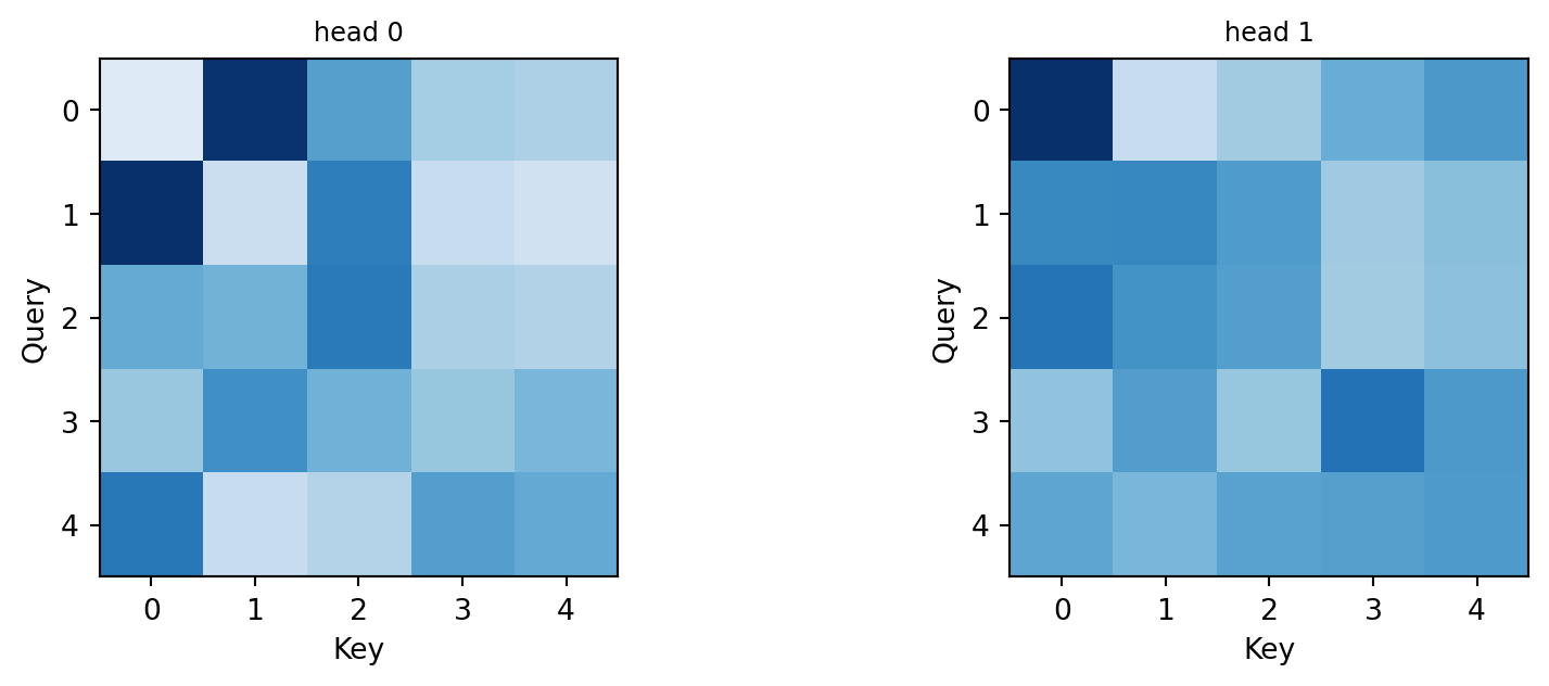
4-4. head마다 다른 곳을 본다
= plt.subplots(1 , H, figsize= (4.6 * H, 3.4 ))for h in range (H):= wh[0 , h].detach().numpy()= axes[h].imshow(M, cmap= 'Blues' , vmin= 0 , vmax= M.max ())f'head { h} ' , fontsize= 9 )'Key' ); axes[h].set_ylabel('Query' ); plt.show()
학습 전(무작위 초기화)이라 아직 의미 있는 패턴은 없다. 학습된 모델에서는 head마다 어순·주어–동사·같은 단어 반복 같은 서로 다른 관계 를 담게 된다.
5. 패딩 마스크와 인과 마스크를 함께 쓰기
10주차에서 만든 패딩 마스크를 어텐션에 연결한다.
= torch.tensor([[1 , 1 , 1 , 0 , 0 ], # 문장 1: 3토큰 1 , 1 , 1 , 1 , 1 ]]) # 문장 2: 5토큰 print ('패딩 마스크 (1=진짜 토큰): \n ' , attn_mask_pad.numpy())# (B, 1, 1, T) 로 만들어 Key 방향에 걸리게 한다 = (attn_mask_pad == 0 )[:, None , None , :]= torch.triu(torch.ones(T, T, dtype= torch.bool ), 1 )[None , None ]= pad_block | causal_blockprint (' \n 결합 마스크 shape:' , tuple (combined.shape))print ('문장 1의 마스크 (True=가림): \n ' , combined[0 , 0 ].numpy().astype(int ))
패딩 마스크 (1=진짜 토큰):
 [[1 1 1 0 0]
 [1 1 1 1 1]]

결합 마스크 shape: (2, 1, 5, 5)
문장 1의 마스크 (True=가림):
 [[0 1 1 1 1]
 [0 0 1 1 1]
 [0 0 0 1 1]
 [0 0 0 1 1]
 [0 0 0 1 1]]
= Wq(x).view(B, T, H, d_head).transpose(1 , 2 )= Wk(x).view(B, T, H, d_head).transpose(1 , 2 )= Wv(x).view(B, T, H, d_head).transpose(1 , 2 )= attention(qh2, kh2, vh2, mask= combined)print ('출력 shape:' , tuple (o2.shape))print (' \n 문장 1, head 0의 가중치:' )print (w2[0 , 0 ].detach().numpy().round (3 ))print (' \n 패딩 열(3, 4)의 가중치 합:' , float (w2[0 , :, :, 3 :].sum ()), ' ← 0이어야 한다' )
출력 shape: (2, 2, 5, 4)

문장 1, head 0의 가중치:
[[1.    0.    0.    0.    0.   ]
 [0.819 0.181 0.    0.    0.   ]
 [0.302 0.281 0.417 0.    0.   ]
 [0.26  0.419 0.321 0.    0.   ]
 [0.569 0.189 0.243 0.    0.   ]]

패딩 열(3, 4)의 가중치 합: 0.0  ← 0이어야 한다
print ('nan이 있는가:' , bool (torch.isnan(o2).any ()))print ('문장 1의 행별 가중치 합:' , w2[0 , 0 ].sum (- 1 ).detach().numpy().round (4 ))
nan이 있는가: False
문장 1의 행별 가중치 합: [1. 1. 1. 1. 1.]
패딩 행(3, 4번)도 앞쪽 진짜 토큰을 보고 있으므로 계산 자체는 성립한다. 그 출력은 의미가 없으니 나중에 버리면 된다.
마스크를 Key 방향뿐 아니라 Query 방향에도 걸면, 어떤 행은 볼 수 있는 칸이 하나도 없게 된다. 그 행은 Softmax의 분모가 0이 되어 nan 이 나온다.
= torch.zeros(1 , 4 , 4 , dtype= torch.bool )0 , 2 , :] = True # 2번 행을 통째로 가린다 = torch.randn(1 , 4 , 8 ); k4 = torch.randn(1 , 4 , 8 ); v4 = torch.randn(1 , 4 , 8 )= attention(q4, k4, v4, mask= bad)print ('가중치: \n ' , w_bad[0 ].numpy().round (3 ))print (' \n nan이 있는가:' , bool (torch.isnan(o_bad).any ()))
가중치:
 [[0.314 0.283 0.216 0.187]
 [0.101 0.412 0.125 0.362]
 [  nan   nan   nan   nan]
 [0.106 0.611 0.228 0.056]]

nan이 있는가: True
패딩 마스크는 Key 방향(마지막 축)에만 거는 것이 안전하다.
5.5. 완성 — 어텐션이 어디를 보는지 꺼내 본다
지난주 감성 분류기는 토큰 임베딩을 평균 냈다. 이번에는 어텐션이 가중치를 정하게 한다.
\[\text{평균} = \sum_t \frac{1}{T} X_t
\qquad\longrightarrow\qquad
\text{어텐션} = \sum_t w_t X_t, \quad \textstyle\sum_t w_t = 1\]
가중치 \(w_t\) 를 사람이 정하지 않고 학습으로 얻는다는 것 이 차이의 전부다.
5-5-1. 데이터
import timeimport pandas as pdfrom transformers import AutoTokenizerfrom torch.utils.data import TensorDataset, DataLoader= AutoTokenizer.from_pretrained('klue/bert-base' )= 'https://raw.githubusercontent.com/e9t/nsmc/master/ratings_train.txt' = 'https://raw.githubusercontent.com/e9t/nsmc/master/ratings_test.txt' = pd.read_csv(TRAIN_URL, sep= ' \t ' ).dropna().sample(20000 , random_state= 42 )= pd.read_csv(TEST_URL, sep= ' \t ' ).dropna().sample(5000 , random_state= 42 )= 48 def encode(df):= tok(list (df['document' ]), padding= 'max_length' , truncation= True ,= MAX_LEN, return_tensors= 'pt' )return e['input_ids' ], e['attention_mask' ], torch.tensor(df['label' ].to_numpy())= encode(train_df)= encode(test_df)print ('훈련' , tuple (Xtr.shape), ' 테스트' , tuple (Xte.shape))
훈련 (20000, 48) 테스트 (5000, 48)
5-5-2. 어텐션 풀링 — 가중치를 학습으로 정한다
토큰마다 점수 하나 를 매기고, 마스크를 씌우고, Softmax로 가중치를 만든다. 1절에서 한 계산과 구조가 같다 — Query가 학습되는 벡터 하나일 뿐이다.
class AttnPoolNet(nn.Module):def __init__ (self , vocab_size, d= 64 , n_classes= 2 ):super ().__init__ ()self .emb = nn.Embedding(vocab_size, d, padding_idx= tok.pad_token_id)self .score = nn.Linear(d, 1 ) # 토큰마다 점수 하나 self .fc = nn.Linear(d, n_classes)def forward(self , ids, mask, return_weights= False ):= self .emb(ids) # (B, T, d) = self .score(X).squeeze(- 1 ) # (B, T) = s.masked_fill(mask == 0 , float ('-inf' )) # 패딩은 -inf = s.softmax(dim=- 1 ) # (B, T), 행 합 1 = (X * w.unsqueeze(- 1 )).sum (dim= 1 ) # 가중합 → (B, d) = self .fc(v)return (out, w) if return_weights else out42 )= AttnPoolNet(tok.vocab_size)print ('파라미터 :' , f' { sum (p.numel() for p in model.parameters()):,} ' )= model(Xte[:2 ], Mte[:2 ], return_weights= True )print ('출력' , tuple (o.shape), ' 가중치' , tuple (w.shape))print ('가중치 행 합:' , w.sum (1 ).detach().numpy().round (4 ))
파라미터 : 2,048,195
출력 (2, 2)  가중치 (2, 48)
가중치 행 합: [1. 1.]
5-5-3. 학습
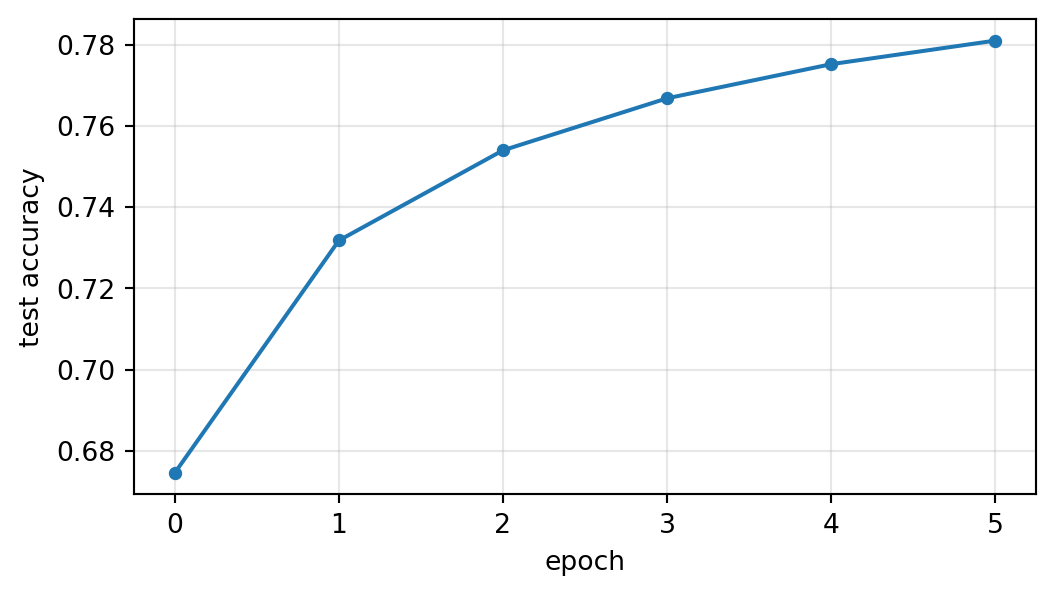
= DataLoader(TensorDataset(Xtr, Mtr, ytr), batch_size= 128 , shuffle= True )= torch.optim.Adam(model.parameters(), lr= 1e-3 )= nn.CrossEntropyLoss()= []= time.time()for ep in range (6 ):for ids, m, y in train_loader:eval ()with torch.no_grad():= (model(Xte, Mte).argmax(1 ) == yte).float ().mean().item()print (f'epoch { ep} test acc { acc:.4f} ' )print (f' \n 학습 시간 { time. time()- t0:.0f} 초' )
epoch 0  test acc 0.6746
epoch 1  test acc 0.7318
epoch 2  test acc 0.7540
epoch 3  test acc 0.7668
epoch 4  test acc 0.7752
epoch 5  test acc 0.7810

학습 시간 5초
= (5.6 , 3.2 ))'o-' , ms= 4 )'epoch' ); plt.ylabel('test accuracy' )= 0.3 ); plt.tight_layout(); plt.show()
지난주 마스크 평균 모형과 정확도가 크게 다르지 않다. 리뷰가 짧고(평균 20토큰 남짓) 데이터가 2만 건이라 평균만으로도 상당히 잘 되기 때문 이다. 어텐션의 값은 여기서는 성능이 아니라 다음 절에 있다.
5-5-4. 모형이 어느 단어를 봤는가
어텐션 가중치는 “모형이 어디를 봤는지”를 그대로 보여 주는 숫자 다. 평균 풀링에서는 볼 수 없던 것이다.
eval ()with torch.no_grad():= model(Xte[:200 ], Mte[:200 ], return_weights= True )= logits.argmax(1 )= list (test_df['document' ])[:200 ]for i in range (6 ):= int (Mte[i].sum ())= W_all[i, :n]= tok.convert_ids_to_tokens(Xte[i, :n])= torch.argsort(w_i, descending= True )[:5 ]= lambda v: '긍정' if v == 1 else '부정' print (f'[정답 { tag(int (yte[i]))} / 예측 { tag(int (pred[i]))} ] { texts[i][:45 ]} ' )print (' 가장 많이 본 토큰:' ,' | ' .join(f' { toks[j]} ( { float (w_i[j]):.3f} )' for j in top.tolist()))print ()
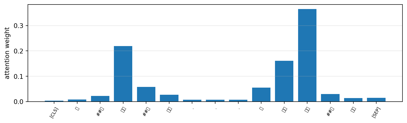
[정답 긍정 / 예측 긍정]  찐한 여운과 함께...내 인생 최고의 미드
   가장 많이 본 토큰: 최고(0.365) | 여운(0.219) | 인생(0.161) | ##과(0.058) | 내(0.055)

[정답 긍정 / 예측 긍정]  기대 이상이다
   가장 많이 본 토큰: ##이다(0.434) | 기대(0.244) | 이상(0.174) | [SEP](0.118) | [CLS](0.030)

[정답 부정 / 예측 부정]  신날 것 없는 애니.
   가장 많이 본 토큰: 없(0.346) | 신(0.236) | 애니(0.175) | ##는(0.066) | [SEP](0.051)

[정답 긍정 / 예측 긍정]  마지막까지 힘을잃지않은 드라마~~
   가장 많이 본 토큰: ##않(0.297) | 마지막(0.202) | ##잃(0.119) | ##을(0.064) | ~(0.060)

[정답 부정 / 예측 부정]  정말아니다. 그냥 뒤끝이 불쾌하고 상황에 대처하는 언니와 순경을 보고 너무 비현실
   가장 많이 본 토큰: 0(0.078) | 그냥(0.067) | ##끝(0.064) | 불쾌(0.058) | ##라(0.054)

[정답 긍정 / 예측 긍정]  영화공사중 도로를 보았는데 에어컨을.. 정말 더웠다.하지만 더글라스오빠연기 압권
   가장 많이 본 토큰: ##공사(0.103) | 정말(0.092) | ##권(0.092) | ##빠(0.086) | ##웠(0.079)
# 한 문장의 가중치를 막대로 = 0 = int (Mte[i].sum ())= tok.convert_ids_to_tokens(Xte[i, :n])= W_all[i, :n].numpy()= (9 , 2.8 ))range (n), w_i)range (n), toks, rotation= 60 , fontsize= 7 )'attention weight' ); plt.grid(alpha= 0.3 , axis= 'y' ); plt.show()print (texts[i])
성능이 아니라 설명 가능성 이다. “왜 이 리뷰를 부정이라고 봤나”에 모형이 “없”, “최악” 이라는 토큰에 가중치를 몰았기 때문” 이라고 답할 수 있다.
프로젝트 진단에서도 같은 질문을 하게 된다 — 모형이 무엇을 보고 판단했는가.
직접 쓴 리뷰 문장을 넣어 예측과 어텐션 가중치를 확인하시오. 모형이 주목한 단어가 납득이 가는가?
= [None ] # ← 문장 두세 개를 적으세요 = tok(my_reviews, padding= True , truncation= True , max_length= MAX_LEN, return_tensors= 'pt' )with torch.no_grad():= model(e['input_ids' ], e['attention_mask' ], return_weights= True )# 위 5-5-4의 출력 코드를 참고해 상위 토큰을 찍어 보세요
예시 보기
= ['배우 연기가 정말 좋았고 여운이 오래 남는다' ,'돈이 아깝다 시간 낭비였음' ,'재미없지 않았다' ]= tok(my_reviews, padding= True , truncation= True , max_length= MAX_LEN, return_tensors= 'pt' )eval ()with torch.no_grad():= model(e['input_ids' ], e['attention_mask' ], return_weights= True )= lo.softmax(1 )for k, s_ in enumerate (my_reviews):= int (e['attention_mask' ][k].sum ())= tok.convert_ids_to_tokens(e['input_ids' ][k, :n])= ww[k, :n]= torch.argsort(w_k, descending= True )[:4 ]print (f' { "긍정" if prob[k,1 ] > 0.5 else "부정" } ( { float (prob[k,1 ]):.3f} ) { s_} ' )print (' ' , ' | ' .join(f' { toks[j]} ( { float (w_k[j]):.3f} )' for j in top.tolist()), ' \n ' )
긍정 (0.978)  배우 연기가 정말 좋았고 여운이 오래 남는다
    여운(0.341) | 좋(0.197) | 정말(0.135) | ##았(0.078)

부정 (0.007)  돈이 아깝다 시간 낭비였음
    돈(0.392) | 낭비(0.268) | 아깝(0.143) | 시간(0.091)

부정 (0.002)  재미없지 않았다
    재미없(0.750) | ##았(0.088) | 않(0.071) | ##지(0.033)
세 번째 문장을 보라. “재미없지 않았다” 는 이중부정이라 긍정인데, 이 모형은 토큰을 가중합 할 뿐 순서를 보지 않으므로 틀리기 쉽다. 토큰끼리 서로를 보게 하려면 self-attention을 층으로 쌓아야 한다 — 다음 주 내용이다.
6. 정리
스코어
Q @ K.transpose(-2,-1) / d**0.5(..., T, T)
행별 Softmax
S.softmax(dim=-1)각 행의 합 = 1
가중합
W @ V(..., T, d)
인과 마스크
torch.triu(torch.ones(T,T,dtype=bool), 1)
가리기
S.masked_fill(mask, float('-inf'))softmax 전에
head 분할
x.view(B,T,H,dh).transpose(1,2)(B, H, T, dh)
head 결합
o.transpose(1,2).reshape(B,T,d)(B, T, d)
한 줄 어텐션
F.scaled_dot_product_attention(q,k,v,is_causal=True)
파라미터
\(4d_{\text{model}}^2\) — head 수와 무관
어텐션 네 줄
\[S = \frac{QK^\top}{\sqrt{d}} \;\to\; S[\text{mask}] = -\infty \;\to\; W = \text{softmax}(S) \;\to\; \text{출력} = WV\]
스스로 확인해 보기
아래 결과를 먼저 예상한 뒤 실행해서 대조한다.
= 4 , 6 , 12 , 3 = torch.randn(B, T, d)= nn.MultiheadAttention(d, H, bias= False , batch_first= True )= m(x, x, x, need_weights= True , average_attn_weights= False )print ('입력 :' , tuple (x.shape))print ('출력 :' , tuple (y.shape))print ('가중치 :' , tuple (w.shape))print ('d_head :' , d // H)print ('파라미터 :' , sum (p.numel() for p in m.parameters()), ' = 4 x' , d, '^2 =' , 4 * d* d)print ()= torch.triu(torch.ones(T, T, dtype= torch.bool ), 1 )= m(x, x, x, attn_mask= mask, need_weights= True , average_attn_weights= False )print ('인과 가중치 위쪽 삼각형 합:' , float (w2[0 , 0 ].triu(1 ).sum ()))print ('마지막 토큰이 보는 칸 수 :' , int ((w2[0 , 0 , - 1 ] > 0 ).sum ()))print ('첫 토큰이 보는 칸 수 :' , int ((w2[0 , 0 , 0 ] > 0 ).sum ()))
입력          : (4, 6, 12)
출력          : (4, 6, 12)
가중치        : (4, 3, 6, 6)
d_head        : 4
파라미터      : 576  = 4 x 12 ^2 = 576

인과 가중치 위쪽 삼각형 합: 0.0
마지막 토큰이 보는 칸 수  : 6
첫 토큰이 보는 칸 수      : 1